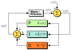
Description of the PID Algorithm
Ut = Kpe(t) + Ki ∫ e(τ) dτ + Kd(de/dt)e(t)
A familiar example of a control loop is the action taken when adjusting hot and cold faucets to fill a container with water at a desired temperature by mixing hot and cold water. The person touches the water in the container as it fills to sense its temperature. Based on this feedback they perform a control action by adjusting the hot and cold faucets until the temperature stabilizes as desired.
The sensed water temperature is the process variable (PV). The desired temperature is called the setpoint (SP). The input to the process (the water valve position), and the output of the PID controller, is called the manipulated variable (MV) or the control variable (CV). The difference between the temperature measurement and the setpoint is the error (e) and quantifies whether the water in the container is too hot or too cold and by how much.
After measuring the temperature (PV), and then calculating the error, the controller decides how much to change the tap position (MV). Because the taps can be adjusted for anything from cool water through to very hot, this is an example of proportional control. In the event that water in the container is not heating quickly enough, the controller may try to speed up the process by opening up the hot water valve quite wide for a while. This is an example of derivative action. If the temperature of the container is settling out too low, despite a good flow of warm water, the controller may open the hot valve more and more as time goes by. This is an example of an integral control.
Making a change that is too large when the error is small will lead to overshoot. If the controller were to repeatedly make changes that were too large and repeatedly overshoot the target, the output would oscillate around the setpoint in either a constant, growing, or decaying sinusoid. If the amplitude of the oscillations increase with time then the system is unstable, whereas if they decrease the system is stable. If the oscillations remain at a constant magnitude the system is marginally stable.
In the interest of achieving a gradual convergence to the desired temperature (SP), the controller may damp the anticipated future oscillations by tempering its adjustments, or reducing the loop gain.
If a controller starts from a stable state with zero error (PV = SP), then further changes by the controller will be in response to changes in other measured or unmeasured inputs to the process that affect the process, and hence the PV. Variables that affect the process other than the MV are known as disturbances. Generally controllers are used to reject disturbances and to implement setpoint changes. Changes in feedwater temperature constitute a disturbance to the faucet temperature control process.
In theory, a controller can be used to control any process which has a measurable output (PV), a known ideal value for that output (SP) and an input to the process (MV) that will affect the relevant PV. Controllers are used in industry to regulate temperature, pressure, flow rate, chemical composition, weight, position, speed and practically every other variable for which a measurement exists.
Finally, at the end there is a description of the Ziegler-Nichols Closed Loop Tuning method. I have used this a little but it has not been my most effective method. It helps for a quick tune.
Proportional Contol (gain)
The first element of PID control to be developed is Proportional control. The equation is simple:
- error = measurement - setpoint (direct action)
- or
- error = setpoint - measurement (reverse action)
Note the action may be either direct or reverse. In a direct acting control loop an increase in the process measurement causes an increase in the ouput to the final control element.
The proportional only equation is:
- output = gain x error + bias
- or
- Pout = Kpe(t)
- Where
- Pout = Proportional response
- Kp = Proportional gain
- ∫ = Integral, from time 0 to present
- e = Error, SP - PV
- t = Instantaneous time (minutes)
The bias is sometimes known as the manual reset. Some control systems (such as Foxboro products, use proportional band rather than gain. The proportional band and the gain are related by:
Gain is the ratio of the change in the output to the change in the input.
![]()
Proportional band is the amount the input would have to change in order to cause the output to move from 0 to 100% (or vice versa)
With proportional only control the controller will not bring the process measurement to the setpoint with out a manual adjustment to the bias (or manual reset) term of the equation. In the early days of control the operator, upon observing an offset in the control loop would correct the offset by manually "reseting" the controller (adjusting the bias).
Integral Control (automatic reset)
The contribution from the integral term is proportional to both the magnitude of the error and the duration of the error. The integral in a PID controller is the sum of the instantaneous error over time and gives the accumulated offset that should have been corrected previously. The accumulated error is then multiplied by the integral gain (Ki) and added to the controller output.
Rather than to require that the operator "manually reset" the control loop whenever there was a load change control functions were developed to "automatically reset" the controller by adjusting the bias term when ever there was an error. This "automatic reset" is also known simply as "reset" or as "integral".
The variable of integration takes on values from time 0 to the present, in minutes. The most common way to implement integral mode in analog controllers is to use a positive feedback into the output.
The equation for PI control is:
- Iout = Ki ∫ e(τ) dτ
- Where
- Ki = Integral gain
- e(τ) = Error integral
- dτ = Derivative integral
The amount of reset used is measured in terms of "reset time" in minutes or its inverse, "reset rate" in repeats per minute. The following test can be perfored on a controller which is not connected to the process:
- an adjustable signal is connected to the input.
- the output is indicated or recorded.
- wtih the controller manual the setpoint and the input are set to the same value.
- the controller is switched to automatic. Becuase the error is zero, the output does not change.
- The input to the controller is changed by a small amount. The output will move suddenly due to the gain. The output will continue to change at a constant rate. The time is measured from the time of the intitial change until the time that the instant change is repeated by the constant movement. The repeat time, or reset time, is the time it takes for the reset effect to repeat (or move the output the same amount as) the gain effect. Its inverse is reset rate, measured in repeats per minute.
Derivative Control (Pre-Act (TM) or Rate)
The third term of PID control is derivative, also known as Pre-Act (trade mark of Taylor Instrument Companies, now ABB), and rate.
The derivative term looks at the rate of change of the input and adjusts the output based on the rate of change. The derivative function can either use the time derivative of the error, which would include changes in the setpoint, or of the measurement only, excluding setpoint changes.
The equation for the derivative contribution (assuming derivative on error) is:
- Dout = Kd(de/dt)e(t)
- Where
- Kd= Derivative Gain
- dt= Derivative time (minutes)
- de= Derivative error
- e = error
- t = instantaneous time
The amount of derivative used is measured in minutes of derivative. To illustrate the meaning of minutes of derivative, consider the following open loop test:
- Connect a signal generator with a ramp cability to the input of a controller. The controller output is connected to a recorder. Configure the controller with some gain, no reset, and no derivative.
- With a constant output from the signal generator and the controller in manual, adjust the setpoint to be equal to the input from the signal generator.
- Place the controller into automatic mode.
- Start the ramp.
- Later stop the ramp.
- Repeat the above steps with some derivative. Compare the trend records of the controller's input and output.
On the trend record (right) note that when the ramp is started, with no derivative (dashed line) the output ramps up due to the change in input and the gain. Using derivative (solid line) the output jumps up, rises in a ramp, then jumps down. The difference in time between the solid line and the dashed line represents the amount of derivative, in units of time (usually minutes).
Putting it together: PID control
Combining the three elements, gain, integral, and derivative, we have the equation:
- Ut = Kpe(t) + Ki ∫ e(τ) dτ + Kd(de/dt)e(t)
- Where
- Pout = Proportional response
- Kp = Proportional gain
- ∫ = Integral, from time 0 to present
- e = Error, SP - PV
- t = Instantaneous time (minutes)
- Ki = Integral gain
- e(τ) = Error integral
- dτ = Derivative integral
- Kd= Derivative Gain
- dt= Derivative time (minutes)
- de= Derivative error
Shown graphically to the right.
Note that in the equation the gain is multiplied by all three terms. This is important for the PID equation to be able to be tuned by any of the standard tuning methods.
Manual tuning
Before starting, test the linearity of the control equipment. Is there a linear relationship between the control and the process? Graph the control at 3 to 4 points in the span, like 25, 50,and 75 percent, and graph the process response. The relationship between the control and response is a good place to start for Kp. The time between control change and process final response will be a good start for integral time.
If the system must remain online, one tuning method is to first set Ki and Kd values to zero. Increase the Kp until the output of the loop oscillates, then the Kp should be set to approximately half of that value for a "quarter amplitude decay" type response. Then increase Ki until any offset is corrected in sufficient time for the process. However, too much will cause instability. Finally, increase Kd, if required, until the loop is acceptably quick to reach its reference after a load disturbance. Careful, too much Kd will cause excessive response and overshoot. A fast PID loop tuning usually overshoots slightly to reach the setpoint more quickly. Some systems cannot accept overshoot, in which case an over-damped closed-loop system is required, which will require a Kp setting significantly less than half that of the Kp setting that was causing oscillation.
Ziegler-Nichols Closed Loop Tuning
The Ziegler-Nichols Closed Loop method is one of the more common methods used to tune control loops. It was first introduced in a paper published in 1942 by J.G. Ziegler and N.B. Nichols, both of whom at the time worked for the Taylor Instrument Companies of Rochester, NY.
The open loop method is useful for most process control loops. To use the method the loop is tested with the controller in automatic. The Closed Loop method determines the gain at which a loop with proportional only control will oscillate, and then derives the controller gain, reset, and derivative values from the gain at which the oscillations are sustained and the period of oscillation at that gain.
The ZN Closed Loop method should produce tuning parameters with will obtain quarter wave decay. This is considered good tuning but is not necessarily optimum tuning.
Steps
- First, note whether the required proportional control gain is positive or negative. To do so, step the input u up (increased) a little, under manual control, to see if the resulting steady state value of the process output has also moved up (increased). If so, then the steady-state process gain is positive and the required Proportional control gain, Kc, has to be positive as well.
- Turn the controller to P-only mode, i.e. turn both the Integral and Derivative modes off.
- Turn the controller gain, Kc, up slowly (more positive if Kc was decided to be so in step 1, otherwise more negative if Kc was found to be negative in step 1) and observe the output response. Note that this requires changing Kc in step increments and waiting for a steady state in the output, before another change in Kc is implemented.
- When a value of Kc results in a sustained periodic oscillation in the output (or close to it), mark this critical value of Kc as Ku, the ultimate gain. Also, measure the period of oscillation, Pu, referred to as the ultimate period. ( Hint: for the system A in the PID simulator, Ku should be around 0.7 and 0.8 )
- Using the values of the ultimate gain, Ku, and the ultimate period, Pu, Ziegler and Nichols prescribes the following values for Kc, tI and tD, depending on which type of controller is desired:
Ziegler-Nichols Tuning Chart:
|
|
|
|
|
|
|
|
||
|
|
|
|
|
|
|
|
|
|